Now let’s continue to understand the recent g-2 result. Last time we briefly touched upon how current loops respond to an external magnetic field, and why electrons and muons fall into this category due to their spin. Now let us sketch how the value is actually related to the spin.

Classical value

Just like the classical current loop, or the classical approximation of hydrogen, the magnetic dipole moment is related to how fast the target rotates – in the case of electron or muon its spin. In quantum mechanics, the two values are simply related. The ratio between the magnetic moment and the spin, in the unit of \(\frac{e}{2m}\) (half-of-charge-mass-ratio) is two. This weird looking unit can be further understood qualitatively through a dimensional analysis – a simple yet powerful device we physicists are very proud of:¹ the potential energy stored in the magnetic moment - magnetic field system is proportional to the magnitude of both. More specifically, its the inner product of the two (pseudo) vectors \(V(x) = - \mathbf{\mu} \cdot \mathbf{B}\). In natural unit (\(c=1, \hbar = 1\)) energy potential has the same unit as mass, and magnetic field (due to being the curl of a vector potential) has mass dimension two, so this gives the magnetic dipole moment mass dimension \(-1\). Given that this is a low energy process, the only relevant energy scale is the electron (or muon) mass, so it’s proportional to \(1/m\). On top of that, we know that with the same spin, the more electric charge it carries, the larger is the “current” in the current loop picture, so it should also be proportional to the electric charge of electron (or muon). Lastly, the faster it spins the bigger is the “current”. So we get

\begin{align} \mathbf{\mu} \propto \frac{e}{m} \mathbf{S} \end{align} where \(S\) is the spin of the electron (or muon.) Using the device called Feynman diagram, we can represent this process as

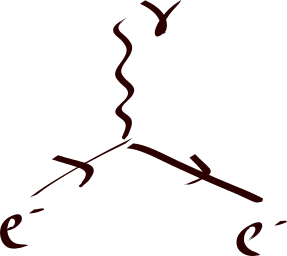
The normalization of the expression is the so-called Landé g-factor: \(\mathbf{\mu} = g \frac{e}{2m} \mathbf{S}\), and its classical value is \(g=2\).

Quantum corrections

However, as is understood now, “on-shell” particles – particles whose energy and momentum is related by their mass hence could have long lifetime – are not the only building blocks in our universe. In a theory developed spanning from the 20s to 50s called quantum field theory (quantum electrodynamics, or QED, to be specific,) it is proposed that virtual particles, particle states that have very short lifetime and whose “mass” could be very different from their on-shell counterparts, can momentarily appear out of vacuum and quickly disappear due to the Heisenberg principle. This revolutionized the way people perceive how fundamental particles interact with each other. However, the theory suffers great problem in making predictions due to a problem related to what is now known as renormalization. Without properly subtracting certain terms and compare with experimental boundary values, the theory suffers infinities here and there, greatly limiting its use. This is so until around 1950s when Richard Feynman, Julian Schwinger, and Shinichiro Tomonaga developed the modern version of the renormalization procedure which was explained by Freeman Dyson. Electron g-2 was the first big test, as the term was predicted by (renormalized) QED and was ready to be compared with the experimental results. This was done in 1948 by Schwinger to show the QED correction to the classical value was about one part out of 1000. When compared to the experimental measurement, this was shown to be consistent up to one part out of 100,000!

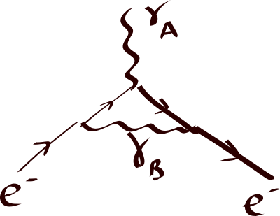
Since electromagnetic fields are all described by photons, the correction computed in the 40s first by Schwinger can be pictorially described as follows. When an electron responds to the magnetic field, it is actually scatters with one of the photons that the magnetic field is “made of”. However, right before the electron scatters with the photon, let’s call it photon A, it can emit another photon (photon B) making both photon B and the electron itself “off-shell”.

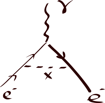
After the off-shell electron scatters with the photon A, and it can “re-absorb” the photon it emitted earlier (photon B) and make itself on-shell again. With the later discovery of other fundamental interactions, weak and strong interactions, photon B can then emit other virtual particles before it gets absorbed by the electron. These effects are of higher order (meaning hierarchically smaller) of course, compared to the leading QED correction. This makes measuring the electron magnetic dipole moment a great way to check for new interactions or particles that couple to electrons (or muons) and photons. The advantage of this approach is that the new particle could be heavy and hard to produce in collider experiments, yet we can measure their contributions without actually produce them on-shell. Brookhaven National Laboratory (BNL) measured the \(g\) factor of \(\mu^-\) up to 0.7 part per million, expressed as ²

\begin{align} \frac{g-2}{2} = 11 659 214 (8)(3) \times 10^{-10}, \end{align} where the two digits in parentheses are the uncertainties in the last digit, with first being statistical uncertainty, and second being systematic. In April, 2021, Fermilab released another result by combining their data and Brookhaven data ³: \begin{align} \frac{g-2}{2} = 116592061(41) \times 10^{-11}. \end{align} with the number in parenthesis the combined uncertainty.

On the other hand, the latest theoretical prediction based on the Standard Model (SM) is \begin{align} \frac{g-2}{2} = 116591810(43) \times 10^{-11}. \end{align}

Comparing the two latest theoretical prediction, and that from the Fermilab + Brookhaven results, one can quantify the disagreement between them to be statistically significant, as \(4.2\) sigma. The chance of this to be purely due to statistical fluctuation is 1 in 40,000!

New physics contribution

There have been a lot of models trying to explain the tension in the last two decades. The rough idea is that the contribution to the magnetic dipole moment should include not only the Standard Model (SM) particles that talk to electrons and muons but also those beyond SM, which couple to muon or photons.

A class of them – the axion models – look particularly appealing due to a few reasons. One of them is that they do not lead to the so-called naturalness problem by themselves. When we study the axion effective field theory (EFT) at low energy, there is parameter space showing that they can address the muon g-2 anomaly without violating any other constraints. This makes a more careful study of the complete theory that generates the EFT very appealing, so we gave it a go in our recent paper. In studying of the UV complete theories, we’ve identified a few issues. We point out that these models are very hard to build without violating the existing experiments. In other words, if these models are the answer to the missing piece that caused the mismatch between the experiment and theoretical prediction, they should come with other particles light enough that have already been observed at other collider experiments. I’ll write more on this in a future post.